
Framing
The threshold is an input
One classifier scores P(rain > h) for any h. Predictions are made on a fixed grid of thresholds with a running minimum, so a higher threshold can never get a higher probability.
Academic · Distributed ML · Data engineering
NUS MSc Data Science for Sustainability · DSA5208 Scalable Distributed Computing · Team of three · October 2026
Eight years of five-minute rain-gauge readings, 48.5 million rows from 91 stations, processed end to end in Spark. The model answers one operational question for any station, time and threshold: how likely is more than h mm of rain in the next 30 minutes?
Singapore’s rain arrives in short, intense bursts. A five-millimetre half-hour happens in fewer than 1 in 100 station-half-hours, which makes it easy to predict “no rain” and hard to predict anything useful.
The brief had two parts: explore how rainfall varies within the year and across 2017 to 2024, then build a Spark MLlib model for the probability that a station records more than h mm in the next 30 minutes. We made the threshold an input of a single classifier, so one model answers for every threshold from 0.2 mm to 60 mm.
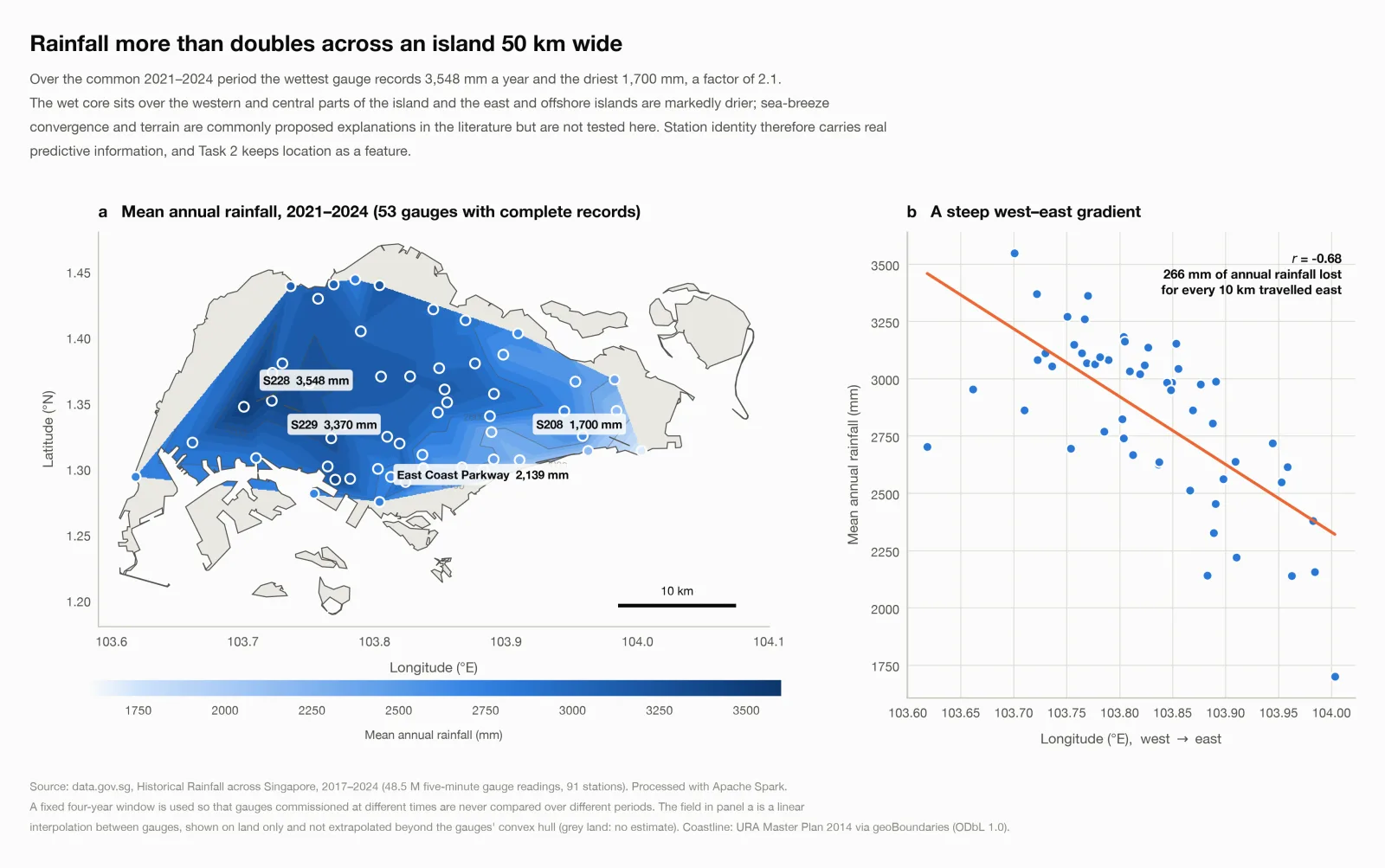
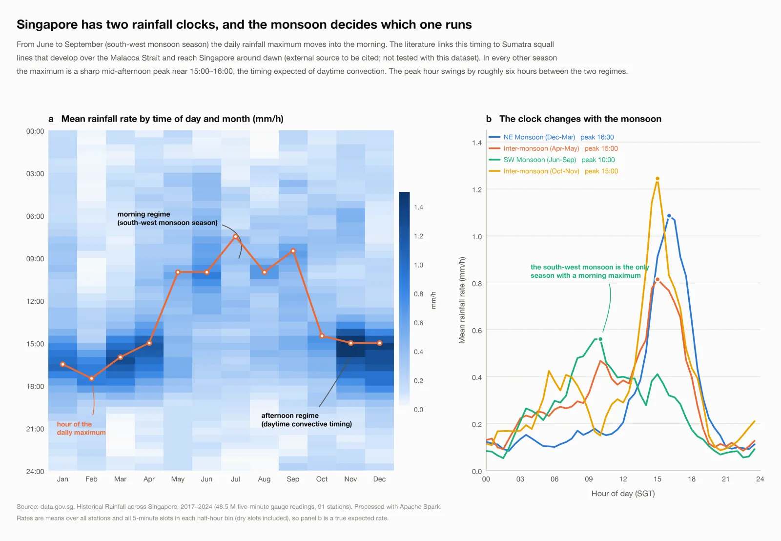
This was a three-person team project. I wrote the first version of the pipeline: ingestion of the raw CSVs into typed Parquet, the Task 1 rainfall-pattern analysis with its tables and figures (including the map and the diurnal-cycle chart below), and the Stage 1 exceedance-probability model with its feature builder, training, evaluation and prediction scripts.
The team then merged our two pipelines into one notebook and added the Stage 2 feature set, the cross-validated model comparison, the scaling study and the Google Cloud Dataproc runs.
Disclosure
The team declared its use of Claude for code, design discussion and drafting in the submitted report. Figures on this page are the project’s own outputs from public data.gov.sg records.
Data moves through three Parquet layers, partitioned by year, so each stage can be rerun or checked on its own.
Bronze
Typed copy of the raw CSVsAn explicit schema, timestamps in Asia/Singapore, nothing dropped yet.
Silver
Cleaned readings and a station tableSnapped to the five-minute grid, de-duplicated, range-checked, faulty gauges removed.
Gold
Features, training sets and predictionsWindow-function features per station and its neighbours, built with a strict time cut-off.
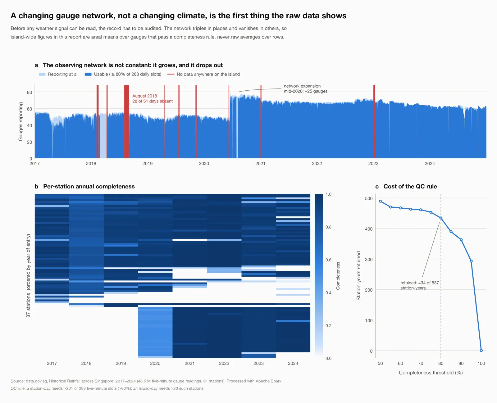
The raw values were clean; the problems were the timestamp grid, gaps and a few broken gauges. A station-month is dropped as a dead gauge when it records under 10% of the network median in a wet month. A day of 100 mm or more is dropped as a spike when it is over four times the wettest gauge within 5 km. Missing readings are never filled with zeros.
Cleaning in numbers
All in 2017, keeping the latest update.
198,544 readings removed.
One gauge logged 749 mm while its neighbours logged 32 mm or less.
Framing
One classifier scores P(rain > h) for any h. Predictions are made on a fixed grid of thresholds with a running minimum, so a higher threshold can never get a higher probability.
Leakage
Every feature uses readings measured at or before five minutes before the prediction time. An independent pandas recomputation checks random rows against the Spark values, and the 2023 rows whose target window reaches into 2024 are dropped.
Sampling
Stage 1 samples by a hash of station, time and threshold, so rare heavy-rain rows are neither over- nor under-sampled. Stage 2 uses inverse-probability weights for its sample.
Validation
Four folds over whole years from 2017 to 2023 compare 25 settings of logistic regression, random forest and gradient-boosted trees. The lowest cross-validated log loss wins, and 2024 is touched once, at the end.
Stage 1, which I first built as standalone scripts, is an interpretable logistic regression on each station’s recent rain and its four nearest gauges, with threshold-by-rain interactions. Stage 2 adds minutes since the last rain, storm trend, three rings of neighbouring gauges, the island-wide wet share and rain so far today. The winning random forest has 100 trees of depth 12 with a Platt calibrator, kept because it helped on held-out 2023 data.
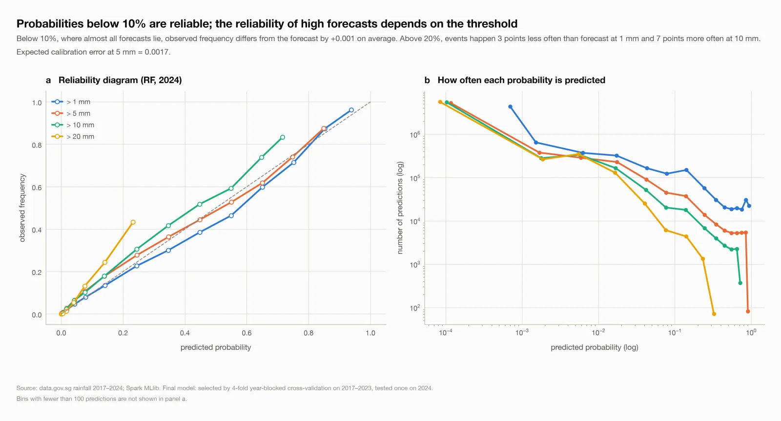
At 5 mm the event rate is 0.84%, so a model that always guesses the base rate scores a PR-AUC of about 0.008. The final model reaches 0.465, about 55 times that.
| Threshold | Event rate | PR-AUC | ROC-AUC | Brier skill |
|---|---|---|---|---|
| 0.5 mm | 3.63% | 0.721 | 0.965 | 0.49 |
| 1 mm | 2.57% | 0.666 | 0.967 | 0.45 |
| 2 mm | 1.69% | 0.587 | 0.965 | 0.39 |
| 5 mm | 0.84% | 0.465 | 0.968 | 0.29 |
| 10 mm | 0.38% | 0.348 | 0.973 | 0.21 |
| 20 mm | 0.10% | 0.183 | 0.981 | 0.10 |
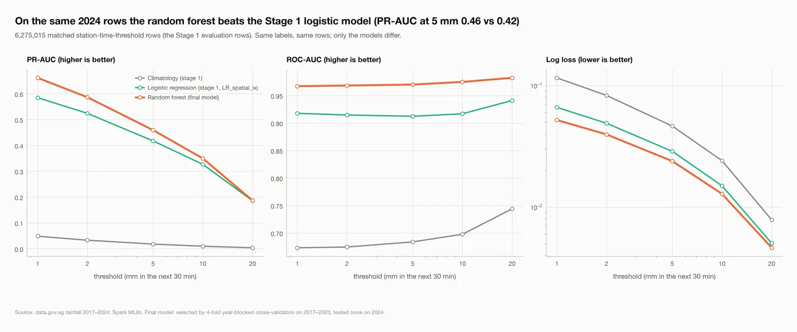
On the matched rows at 20 mm the two models are effectively tied: PR-AUC 0.187 against 0.186, and the logistic model has the slightly better Brier score. Spark’s tree models are not bit-for-bit deterministic, so the third decimal moves between runs.
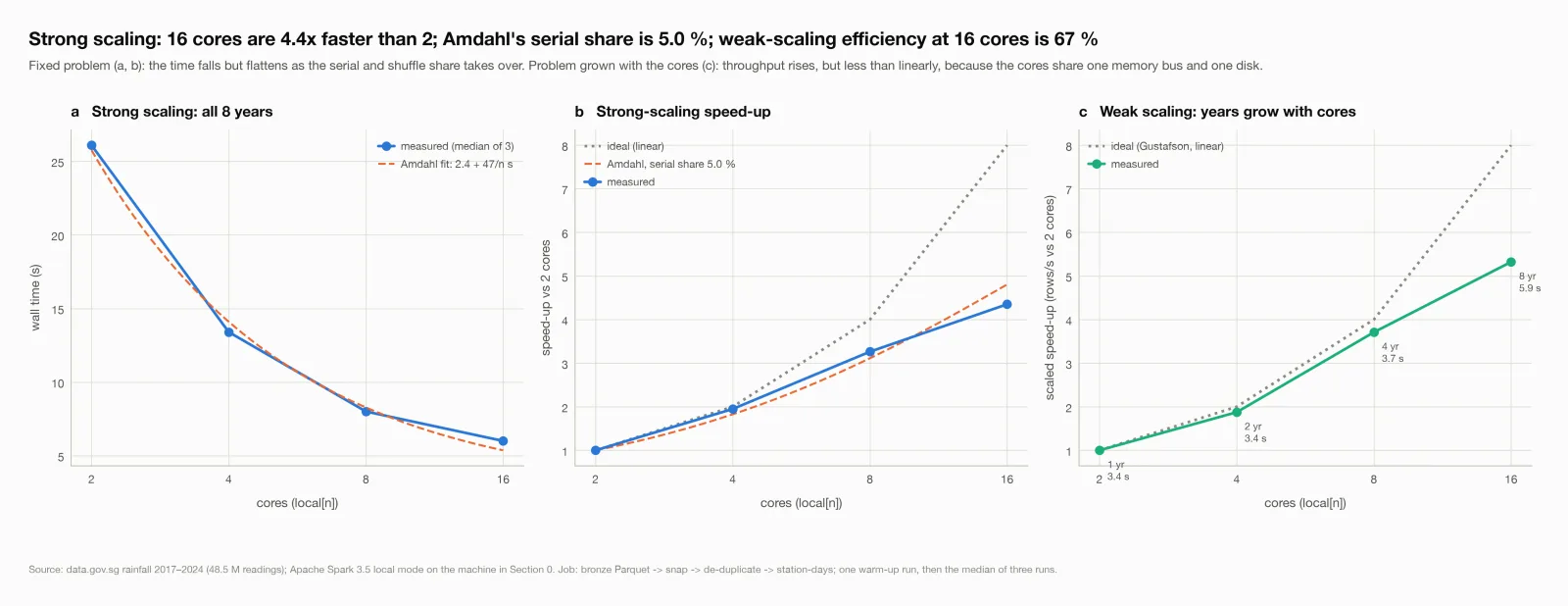
The cleaning step reads all 48.5 million bronze rows, snaps, de-duplicates and aggregates to station-days. On one machine, 16 cores ran it 4.4 times faster than 2. An Amdahl’s-law fit gives a serial share of 5%, so no number of cores could make it more than 20 times faster. On Google Cloud Dataproc, doubling the workers from two to four cut the time from 74.8 s to 37.3 s, because each worker brings its own memory and disk.
The full notebook also ran unchanged on a Dataproc cluster with data on HDFS and reproduced the laptop’s tables exactly and its model scores within Spark’s run-to-run variation (PR-AUC at 5 mm: 0.466 on the laptop, 0.465 on the cluster).
predict(station, time, threshold) as a small scheduled job that scores the next half-hour island-wide.